The new 2.21 version contains significant optimisations (which I should really have included in v2.2), so I thought it would be useful to compare the performance of both the CPU and GPU routines with other micromagnetics software.
Mumax3 (http://mumax.github.io/) runs GPU computations using the CUDA platform, has been around for a number of years and is widely used so I expect it is optimised quite well. It is also a finite difference micromagnetics software so will be very instructive to compare it with Boris.
OOMMF (https://math.nist.gov/oommf/) is a finite difference software that runs on the CPU (although I understand the latest release has extensions for CUDA). OOMMF has been around for a really long time – in fact I used it during my PhD quite a lot – and is a very good software to use as a reference.
To compare the different programs I’ve kept things very simple: run a range of simulation sizes for permalloy using only the demagnetising, exchange, and applied field terms, starting from a uniform magnetisation configuration with a small magnetic field applied perpendicular to it. The simulations are run using exactly the same LLG evaluation methods and same time step for a fixed number of iterations. I’ve used a cubic cellsize of 5 nm throughout. I’ve also disabled any data output after checking all programs do exactly the same thing.
First, Boris (2.21) vs Mumax3 (3.10beta) both in single precision mode. I’ve used the RK4 method with a fixed 500 fs time step and compared them on GTX 980 Ti and GTX 1060 Ti, by changing the problem size from 262,144 points up to 16,777,216 points. I’ve used a number of different “modes” : 3D (simulation space cubic or nearly cubic, e.g. 64x64x64 points up to 256x256x256 points), 3D Thin mode (thin along the z axis, e.g. 256x256x4 up to 2048x2048x4 points), quasi 2D mode (e.g. 512x256x2 up to 4096x2048x2; this is really a 3D computation but can be handled with almost the same level of performance as a 2D computation, and half the scratch space usage compared to a 3D implementation). Finally the 2D mode is also used (512x512x1 up to 4096x4096x1). The reason for including these different modes, with GPU computations a well-optimised convolution pipeline should handle these cases differently. It turns out convolution is a much more complicated problem on the GPU in terms of performance optimisation compared to the CPU.
Here are the results, showing the simulation duration per 400 iterations as a function of problem size (N):
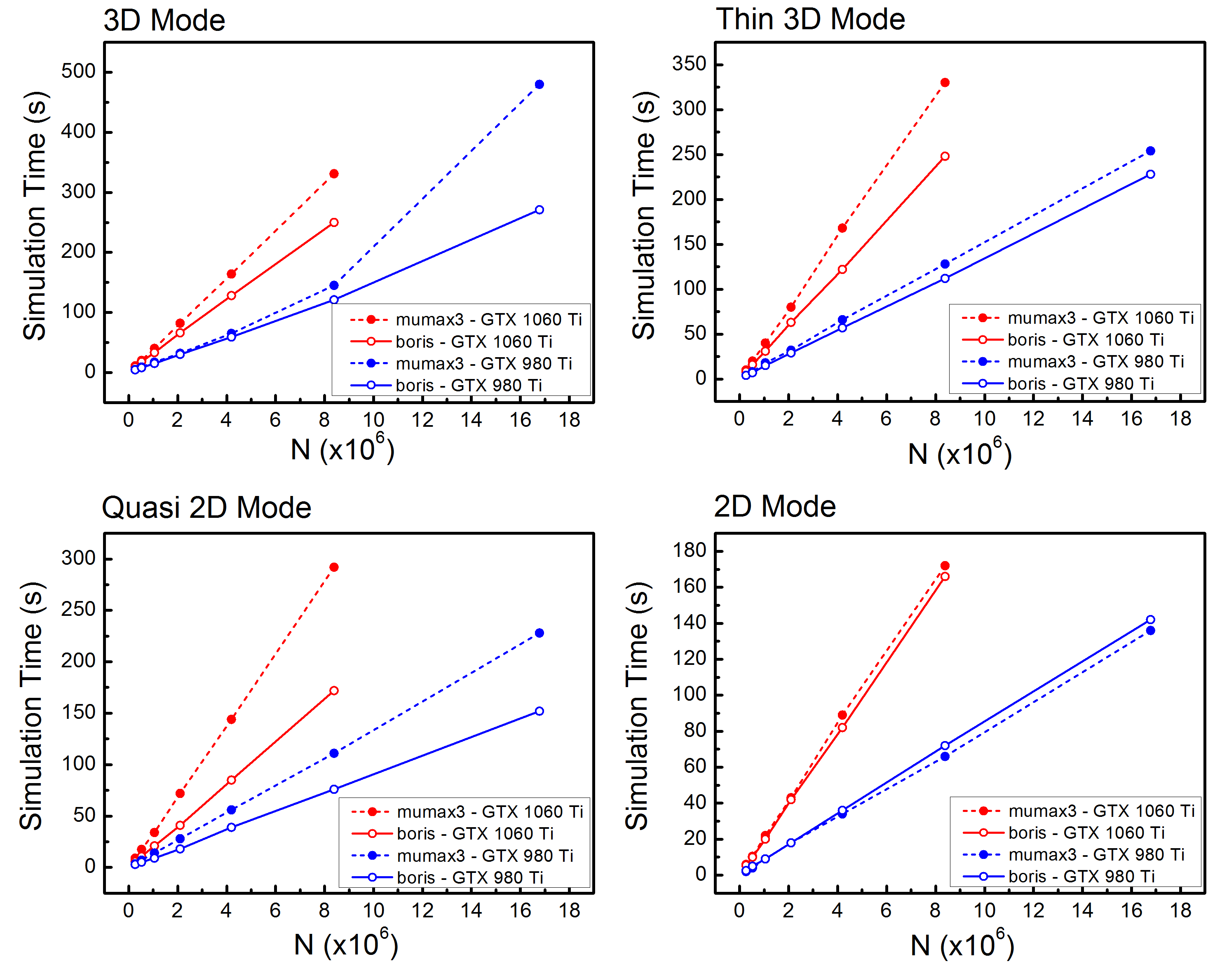
On GTX 1060 Ti Boris is significantly faster than Mumax3 for all 3D modes; the 2D mode is quite close, but this is a much easier problem to optimise so these results are not surprising as both programs do more or less the same thing here.
On GTX 980 Ti the results are closer, although again Boris is faster. The only exception is the 2D mode on GTX 980 Ti where Mumax3 has a slight edge although the difference is close to the benchmarking error. I’m not sure why Mumax3 is really slow at the upper end of the 3D mode on GTX 980 Ti – I’ve verified that point several times!
The mode that really stands out in terms of performance difference is the quasi 2D mode, where Boris is up to 1.7 times faster. The implementation idea in this mode is quite simple, and is very similar to how 3D convolution is implemented on the CPU: the z-axis FFT / kernel multiplication / z-axis IFFT can be rolled into a single step thus saving the need to temporarily store the upper z-axis points. The obvious extension is to apply this technique to the 8, 16, etc. z-axis points cases, although at some point this should become slower due to wasted GPU bandwidth. I will send out for review a large technical publication on Boris in the next few weeks and this is one of the aspects I will include in the discussion (with preprint on arXiv). I also plan to release the source code on GitHub at some point this year.
Finally, Boris (2.21) vs OOMMF (I’ve used 1.2; 2.0 is available but I couldn’t get it to work) both in double precision mode. In Boris the computation mode can be changed seamlessly between CPU and GPU with the cuda console command, so this time I’m running with cuda 0. I’ve had to use the Euler evaluation method with 3 fs time step as the RungeKutta evolver in OOMMF I believe is the RKF45 method, which is an adpative time-step method. Boris also implements this, but for benchmarking purposes it’s better to use a fixed time-step method. Other than this the problem details are as described previously. I’ve compared the programs on the i7 – 4790K processor which has 8 logical processors (4 cores multithreaded), and the i7 – X980 processor which has 12 logical processors (6 cores multithreaded), by changing the problem size from 32,768 points up to 262,144 points.
The results are shown below, where the simulation duration is plotted per 10000 Euler iterations.

For both the 2D and 3D modes Boris runs significantly faster than OOMMF: up to 10 times faster for the smallest problem sizes. I believe this is largely due to an inefficient multithreading model used in OOMMF. On the one hand there is significant overhead associated with it, which explains the order of magnitude difference in performance at the smallest problem sizes, and on the other hand the CPU utilisation is sub-optimal, which explains the still significant difference in performance for the larger problem sizes. For Boris v2.21 I’ve switched to using the FFTW3 library for FFTs, as unsurprisingly it’s faster than my own FFT routines – although it must be implemented carefully; for convolution I’ve found the line-fetch method works best (fetch line, execute FFT, write line back).
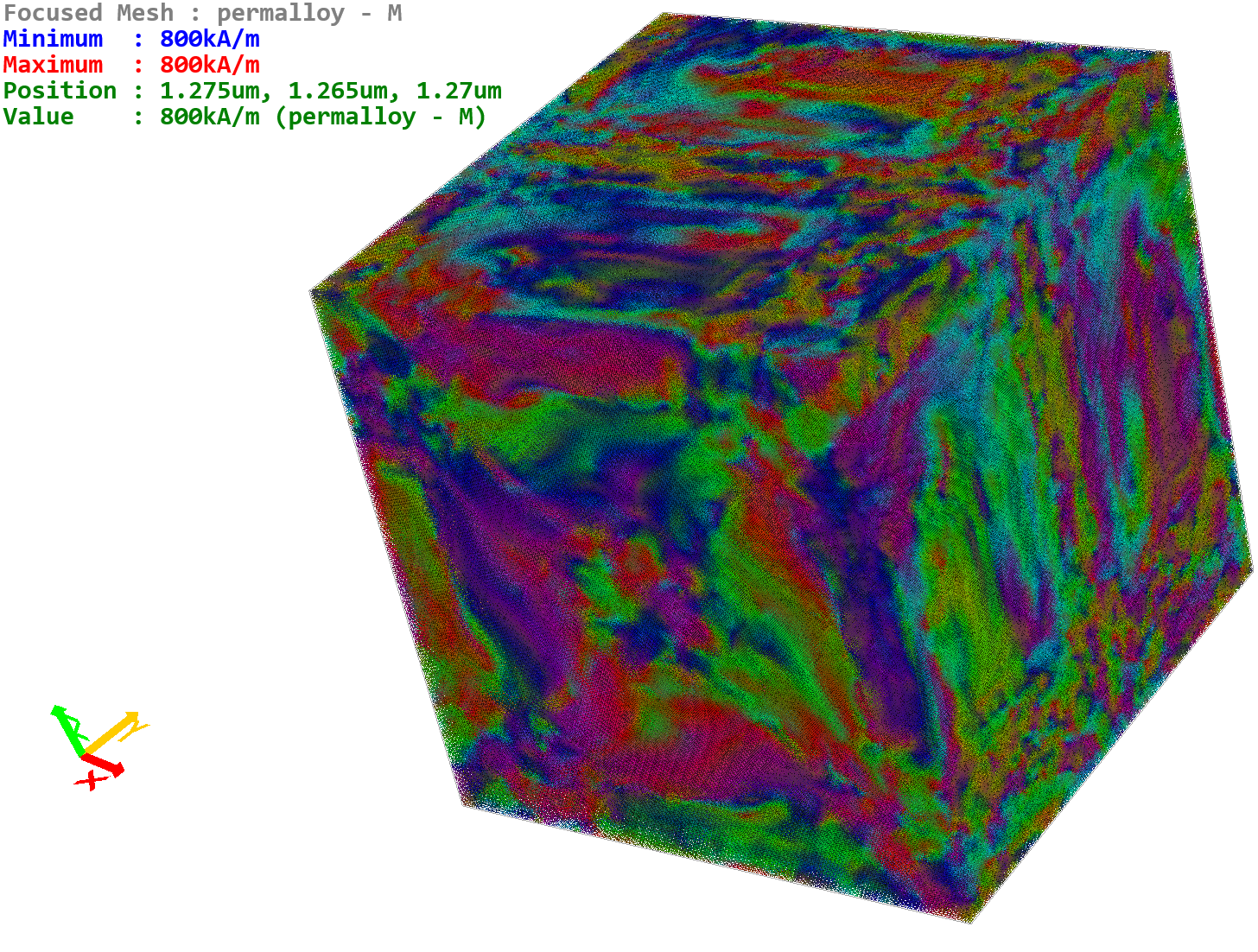
On a final – and somewhat unrelated – note here’s what a 17M point (256x256x256) simulation looks like: